3 Parallel Computing in R

3.1 R Markdown Source

https://raw.githubusercontent.com/cjgeyer/Orientation2018/master/02-parallel.Rmd

3.2 Introduction

The example that we will use throughout this document is simulating the sampling distribution of the MLE for \(\text{Normal}(\theta, \theta^2)\) data.

A lot of this may make make no sense. This is what you are going to graduate school in statistics to learn. But we want a non-toy example.

3.3 Set-Up

# sample size
n <- 10
# simulation sample size
nsim <- 1e4
# true unknown parameter value
# of course in the simulation it is known, but we pretend we don't
# know it and estimate it
theta <- 1

doit <- function(estimator, seed = 42) {
    set.seed(seed)
    result <- double(nsim)
    for (i in 1:nsim) {
        x <- rnorm(n, theta, abs(theta))
        result[i] <- estimator(x)
    }
    return(result)
}

mlogl <- function(theta, x) sum(- dnorm(x, theta, abs(theta), log = TRUE))

mle <- function(x) {
    theta.start <- sign(mean(x)) * sd(x)
    if (all(x == 0) || theta.start == 0)
        return(0)
    nout <- nlm(mlogl, theta.start, iterlim = 1000, x = x)
    if (nout$code > 3)
        return(NaN)
    return(nout$estimate)
}

R function doit simulates nsim datasets, applies an estimator supplied as an argument to the function to each, and returns the vector of results.
R function mlogl is minus the log likelihood of the model in question. We could easily change the code to do another model by changing only this function. (When the code mimics the math, the design is usually good.)
R function mle calculates the estimator by calling R function nlm to minimize it. The starting value sign(mean(x)) * sd(x) is a reasonable estimator because mean(x) is a consistent estimator of \(\theta\) and sd(x) is a consistent estimator of \(\lvert \theta \rvert\).

3.4 Doing the Simulation without Parallelization

3.4.1 Try It

theta.hat <- doit(mle)

3.4.2 Check It

hist(theta.hat, probability = TRUE, breaks = 30)
curve(dnorm(x, mean = theta, sd = theta / sqrt(3 * n)), add = TRUE)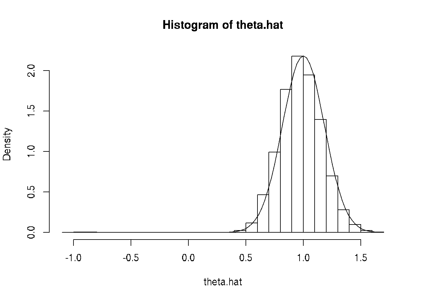

The curve is the PDF of the asymptotic normal distribution of the MLE, which uses the formula \[ I_n(\theta) = \frac{3 n}{\theta^2} \] which you will learn how to calculate when you take a theory course (if you don’t already know).

Looks pretty good. The large negative estimates are probably not a mistake. The parameter is allowed to be negative, so sometimes the estimates come out negative even though the truth is positive. And not just a little negative because \(\lvert \theta \rvert\) is also the standard deviation, so it cannot be small and the model fit the data.

sum(is.na(theta.hat))

## [1] 0

mean(is.na(theta.hat))

## [1] 0

sum(theta.hat < 0, na.rm = TRUE)

## [1] 9

mean(theta.hat < 0, na.rm = TRUE)

## [1] 9e-04

3.4.3 Time It

Now for something new. We will time it.

time1 <- system.time(theta.hat.mle <- doit(mle))
time1

##    user  system elapsed 
##   0.985   0.000   0.985

3.4.4 Time It More Accurately

That’s too short a time for accurate timing. So increase the number of iterations. Also we should probably average over several IID iterations to get a good average. Try again.

nsim <- 1e5
nrep <- 7
time1 <- NULL
for (irep in 1:nrep)
    time1 <- rbind(time1, system.time(theta.hat.mle <- doit(mle)))
time1

##      user.self sys.self elapsed user.child sys.child
## [1,]    10.112    0.000  10.123          0         0
## [2,]    10.175    0.001  10.158          0         0
## [3,]     9.746    0.000   9.726          0         0
## [4,]     9.963    0.000   9.945          0         0
## [5,]     9.665    0.000   9.651          0         0
## [6,]    10.000    0.000   9.987          0         0
## [7,]     9.517    0.000   9.505          0         0

apply(time1, 2, mean)

##    user.self     sys.self      elapsed   user.child    sys.child 
## 9.8825714286 0.0001428571 9.8707142857 0.0000000000 0.0000000000

apply(time1, 2, sd) / sqrt(nrep)

##    user.self     sys.self      elapsed   user.child    sys.child 
## 0.0923298582 0.0001428571 0.0936286266 0.0000000000 0.0000000000

3.5 Parallel Computing With Unix Fork and Exec

3.5.1 Introduction

This method is by far the simplest but

it only works on one computer (using however many simultaneous processes the computer can do), and
it does not work on Windows.

3.5.2 Toy Problem

First a toy problem that does nothing except show that we are actually using different processes.

library(parallel)
ncores <- detectCores()
mclapply(1:ncores, function(x) Sys.getpid(), mc.cores = ncores)

## [[1]]
## [1] 19972
## 
## [[2]]
## [1] 19973
## 
## [[3]]
## [1] 19974
## 
## [[4]]
## [1] 19975
## 
## [[5]]
## [1] 19976
## 
## [[6]]
## [1] 19977
## 
## [[7]]
## [1] 19978
## 
## [[8]]
## [1] 19979

3.5.3 Warning

Quoted from the help page for R function mclapply

It is strongly discouraged to use these functions in GUI or embedded environments, because it leads to several processes sharing the same GUI which will likely cause chaos (and possibly crashes). Child processes should never use on-screen graphics devices.

GUI includes RStudio. If you want speed, then you will have to learn how to use plain old R. The examples in the section on using clusters show that. Of course, this whole document shows that too. (No RStudio was used to make this document.)

3.5.4 Parallel Streams of Random Numbers

To get random numbers in parallel, we need to use a special random number generator (RNG) designed for parallelization.

RNGkind("L'Ecuyer-CMRG")
set.seed(42)
mclapply(1:ncores, function(x) rnorm(5), mc.cores = ncores)

## [[1]]
## [1]  1.11932846 -0.07617141 -0.35021912 -0.33491161 -1.73311280
## 
## [[2]]
## [1] -0.2084809 -1.0341493 -0.2629060  0.3880115  0.8331067
## 
## [[3]]
## [1]  0.001100034  1.763058291 -0.166377859 -0.311947389  0.694879494
## 
## [[4]]
## [1]  0.2262605 -0.4827515  1.7637105 -0.1887217 -0.7998982
## 
## [[5]]
## [1]  0.8584220 -0.3851236  1.0817530  0.2851169  0.1799325
## 
## [[6]]
## [1] -1.1378621 -1.5197576 -0.9198612  1.0303683 -0.9458347
## 
## [[7]]
## [1] -0.04649149  3.38053730 -0.35705061  0.17722940 -0.39716405
## 
## [[8]]
## [1]  1.3502819 -1.0055894 -0.4591798 -0.0628527 -0.2706805

Just right! We have different random numbers in all our jobs. And it is reproducible.

But this may not work like you may think it does. If we do it again we get exactly the same results.

mclapply(1:ncores, function(x) rnorm(5), mc.cores = ncores)

## [[1]]
## [1]  1.11932846 -0.07617141 -0.35021912 -0.33491161 -1.73311280
## 
## [[2]]
## [1] -0.2084809 -1.0341493 -0.2629060  0.3880115  0.8331067
## 
## [[3]]
## [1]  0.001100034  1.763058291 -0.166377859 -0.311947389  0.694879494
## 
## [[4]]
## [1]  0.2262605 -0.4827515  1.7637105 -0.1887217 -0.7998982
## 
## [[5]]
## [1]  0.8584220 -0.3851236  1.0817530  0.2851169  0.1799325
## 
## [[6]]
## [1] -1.1378621 -1.5197576 -0.9198612  1.0303683 -0.9458347
## 
## [[7]]
## [1] -0.04649149  3.38053730 -0.35705061  0.17722940 -0.39716405
## 
## [[8]]
## [1]  1.3502819 -1.0055894 -0.4591798 -0.0628527 -0.2706805

Running mclapply does not change .Random.seed in the parent process (the R process you are typing into). It only changes it in the child processes (that do the work). But there is no communication from child to parent except the list of results returned by mclapply.

This is a fundamental problem with mclapply and the fork-exec method of parallelization. And it has no real solution. You just have to be aware of it.

If you want to do exactly the same random thing with mclapply and get different random results, then you must change .Random.seed in the parent process, either with set.seed or by otherwise using random numbers in the parent process.

3.5.5 The Example

We need to rewrite our doit function

to only do 1 / ncores of the work in each child process,
to not set the random number generator seed, and
to take an argument in some list we provide.

doit <- function(nsim, estimator) {
    result <- double(nsim)
    for (i in 1:nsim) {
        x <- rnorm(n, theta, abs(theta))
        result[i] <- estimator(x)
    }
    return(result)
}

3.5.6 Try It

mout <- mclapply(rep(nsim / ncores, ncores), doit,
    estimator = mle, mc.cores = ncores)
lapply(mout, head)

## [[1]]
## [1] 0.9051972 0.9589889 0.9799828 1.1347548 0.9090886 0.9821320
## 
## [[2]]
## [1] 0.8317815 1.3432331 0.7821308 1.2010078 0.9792244 1.1148521
## 
## [[3]]
## [1] 0.8627829 0.9790400 1.1787975 0.7852431 1.2942963 1.0768396
## 
## [[4]]
## [1] 1.0422013 0.9166641 0.8326720 1.1864809 0.9609456 1.3137716
## 
## [[5]]
## [1] 0.8057316 0.9488173 1.0792078 0.9774531 0.8106612 0.8403027
## 
## [[6]]
## [1] 1.0156983 1.0077599 0.9867766 1.1643493 0.9478923 1.1770221
## 
## [[7]]
## [1] 1.2287013 1.0046353 0.9560784 1.0354414 0.9045423 0.9455714
## 
## [[8]]
## [1] 0.7768910 1.0376265 0.8830854 0.8911714 1.0288567 1.1609360

3.5.7 Check It

Seems to have worked.

length(mout)

## [1] 8

sapply(mout, length)

## [1] 12500 12500 12500 12500 12500 12500 12500 12500

lapply(mout, head)

## [[1]]
## [1] 0.9051972 0.9589889 0.9799828 1.1347548 0.9090886 0.9821320
## 
## [[2]]
## [1] 0.8317815 1.3432331 0.7821308 1.2010078 0.9792244 1.1148521
## 
## [[3]]
## [1] 0.8627829 0.9790400 1.1787975 0.7852431 1.2942963 1.0768396
## 
## [[4]]
## [1] 1.0422013 0.9166641 0.8326720 1.1864809 0.9609456 1.3137716
## 
## [[5]]
## [1] 0.8057316 0.9488173 1.0792078 0.9774531 0.8106612 0.8403027
## 
## [[6]]
## [1] 1.0156983 1.0077599 0.9867766 1.1643493 0.9478923 1.1770221
## 
## [[7]]
## [1] 1.2287013 1.0046353 0.9560784 1.0354414 0.9045423 0.9455714
## 
## [[8]]
## [1] 0.7768910 1.0376265 0.8830854 0.8911714 1.0288567 1.1609360

Plot it.

theta.hat <- unlist(mout)
hist(theta.hat, probability = TRUE, breaks = 30)
curve(dnorm(x, mean = theta, sd = theta / sqrt(3 * n)), add = TRUE)

3.5.8 Time It

time4 <- NULL
for (irep in 1:nrep)
    time4 <- rbind(time4, system.time(theta.hat.mle <-
        unlist(mclapply(rep(nsim / ncores, ncores), doit,
            estimator = mle, mc.cores = ncores))))
time4

##      user.self sys.self elapsed user.child sys.child
## [1,]     0.007    0.012   2.191     14.063     0.217
## [2,]     0.001    0.016   2.733     18.288     0.164
## [3,]     0.003    0.016   3.156     20.357     0.240
## [4,]     0.003    0.016   3.093     20.051     0.200
## [5,]     0.001    0.016   3.091     20.264     0.260
## [6,]     0.000    0.019   3.132     20.185     0.247
## [7,]     0.002    0.016   3.079     20.126     0.236

apply(time4, 2, mean)

##    user.self     sys.self      elapsed   user.child    sys.child 
##  0.002428571  0.015857143  2.925000000 19.047714286  0.223428571

apply(time4, 2, sd) / sqrt(nrep)

##    user.self     sys.self      elapsed   user.child    sys.child 
## 0.0008689661 0.0007693093 0.1337486983 0.8739731857 0.0123901980

We got the desired speedup. The elapsed time averages

apply(time4, 2, mean)["elapsed"]

## elapsed 
##   2.925

with parallelization and

apply(time1, 2, mean)["elapsed"]

##  elapsed 
## 9.870714

without parallelization. But we did not get an 8-fold speedup with 8 cores. There is a cost to starting and stopping the child processes. And some time needs to be taken from this number crunching to run the rest of the computer. However, we did get a 3.4-fold speedup. If we had more cores, we could do even better.

3.6 The Example With a Cluster

3.6.1 Introduction

This method is more complicated but

it works on clusters like the ones at LATIS (College of Liberal Arts Technologies and Innovation Services) or at the Minnesota Supercomputing Institute.
according to the documentation, it does work on Windows.

3.6.2 Toy Problem

First a toy problem that does nothing except show that we are actually using different processes.

library(parallel)
ncores <- detectCores()
cl <- makePSOCKcluster(ncores)
parLapply(cl, 1:ncores, function(x) Sys.getpid())

## [[1]]
## [1] 20000
## 
## [[2]]
## [1] 20009
## 
## [[3]]
## [1] 20018
## 
## [[4]]
## [1] 20027
## 
## [[5]]
## [1] 20036
## 
## [[6]]
## [1] 20045
## 
## [[7]]
## [1] 20054
## 
## [[8]]
## [1] 20063

stopCluster(cl)

This is more complicated in that

first you you set up a cluster, here with makePSOCKcluster but not everywhere — there are a variety of different commands to make clusters and the command would be different at LATIS or MSI — and
at the end you tear down the cluster with stopCluster.

Of course, you do not need to tear down the cluster before you are done with it. You can execute multiple parLapply commands on the same cluster.

There are also a lot of other commands other than parLapply that can be used on the cluster. We will see some of them below.

3.6.3 Parallel Streams of Random Numbers

cl <- makePSOCKcluster(ncores)
clusterSetRNGStream(cl, 42)
parLapply(cl, 1:ncores, function(x) rnorm(5))

## [[1]]
## [1] -0.93907708 -0.04167943  0.82941349 -0.43935820 -0.31403543
## 
## [[2]]
## [1]  1.11932846 -0.07617141 -0.35021912 -0.33491161 -1.73311280
## 
## [[3]]
## [1] -0.2084809 -1.0341493 -0.2629060  0.3880115  0.8331067
## 
## [[4]]
## [1]  0.001100034  1.763058291 -0.166377859 -0.311947389  0.694879494
## 
## [[5]]
## [1]  0.2262605 -0.4827515  1.7637105 -0.1887217 -0.7998982
## 
## [[6]]
## [1]  0.8584220 -0.3851236  1.0817530  0.2851169  0.1799325
## 
## [[7]]
## [1] -1.1378621 -1.5197576 -0.9198612  1.0303683 -0.9458347
## 
## [[8]]
## [1] -0.04649149  3.38053730 -0.35705061  0.17722940 -0.39716405

parLapply(cl, 1:ncores, function(x) rnorm(5))

## [[1]]
## [1] -2.1290236  2.5069224 -1.1273128  0.1660827  0.5767232
## 
## [[2]]
## [1] 0.03628534 0.29647473 1.07128138 0.72844380 0.12458507
## 
## [[3]]
## [1] -0.1652167 -0.3262253 -0.2657667  0.1878883  1.4916193
## 
## [[4]]
## [1]  0.3541931 -0.6820627 -1.0762411 -0.9595483  0.0982342
## 
## [[5]]
## [1]  0.5441483  1.0852866  1.6011037 -0.5018903 -0.2709106
## 
## [[6]]
## [1] -0.57445721 -0.86440961 -0.77401840  0.54423137 -0.01006838
## 
## [[7]]
## [1] -1.3057289  0.5911102  0.8416164  1.7477622 -0.7824792
## 
## [[8]]
## [1]  0.9071634  0.2518615 -0.4905999  0.4900700  0.7970189

We see that clusters do not have the same problem with continuing random number streams that the fork-exec mechanism has.

Using fork-exec there is a parent process and child processes (all running on the same computer) and the child processes end when their work is done (when mclapply finishes).
Using clusters there is a master process and worker processes (possibly running on many different computers) and the worker processes end when the cluster is torn down (with stopCluster).

So the worker processes continue and each remembers where it is in its random number stream (each has a different random number stream).

3.6.4 The Example on a Cluster

3.6.4.1 Set Up

Another complication of using clusters is that the worker processes are completely independent of the master. Any information they have must be explicitly passed to them.

This is very unlike the fork-exec model in which all of the child processes are copies of the parent process inheriting all of its memory (and thus knowing about any and all R objects it created).

So in order for our example to work we must explicitly distribute stuff to the cluster.

clusterExport(cl, c("doit", "mle", "mlogl", "n", "nsim", "theta"))

Now all of the workers have those R objects, as copied from the master process right now. If we change them in the master (pedantically if we change the R objects those names refer to) the workers won’t know about it. They only would make changes if code were executed on them to do so.

3.6.4.2 Try It

So now we are set up to try our example.

pout <- parLapply(cl, rep(nsim / ncores, ncores), doit, estimator = mle)

3.6.4.3 Check It

Seems to have worked.

length(pout)

## [1] 8

sapply(pout, length)

## [1] 12500 12500 12500 12500 12500 12500 12500 12500

lapply(pout, head)

## [[1]]
## [1] 1.0079313 0.7316543 0.4958322 0.7705943 0.7734226 0.6158992
## 
## [[2]]
## [1] 0.9589889 0.9799828 1.1347548 0.9090886 0.9821320 1.0032531
## 
## [[3]]
## [1] 1.3432331 0.7821308 1.2010078 0.9792244 1.1148521 0.9269000
## 
## [[4]]
## [1] 0.9790400 1.1787975 0.7852431 1.2942963 1.0768396 0.7546295
## 
## [[5]]
## [1] 0.9166641 0.8326720 1.1864809 0.9609456 1.3137716 0.9832663
## 
## [[6]]
## [1] 0.9488173 1.0792078 0.9774531 0.8106612 0.8403027 1.1296857
## 
## [[7]]
## [1] 1.0077599 0.9867766 1.1643493 0.9478923 1.1770221 1.2789464
## 
## [[8]]
## [1] 1.0046353 0.9560784 1.0354414 0.9045423 0.9455714 1.0312553

Plot it.

theta.hat <- unlist(mout)
hist(theta.hat, probability = TRUE, breaks = 30)
curve(dnorm(x, mean = theta, sd = theta / sqrt(3 * n)), add = TRUE)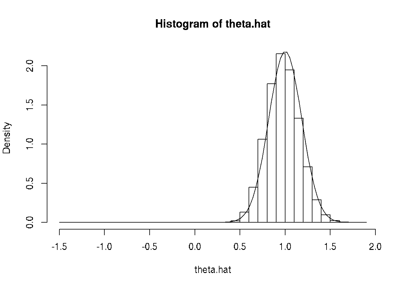

3.6.4.4 Time It

time5 <- NULL
for (irep in 1:nrep)
    time5 <- rbind(time5, system.time(theta.hat.mle <-
        unlist(parLapply(cl, rep(nsim / ncores, ncores),
            doit, estimator = mle))))
time5

##      user.self sys.self elapsed user.child sys.child
## [1,]     0.007    0.000   3.366          0         0
## [2,]     0.003    0.004   3.319          0         0
## [3,]     0.005    0.000   3.346          0         0
## [4,]     0.000    0.006   3.350          0         0
## [5,]     0.006    0.000   3.308          0         0
## [6,]     0.003    0.004   3.376          0         0
## [7,]     0.002    0.004   3.261          0         0

apply(time5, 2, mean)

##   user.self    sys.self     elapsed  user.child   sys.child 
## 0.003714286 0.002571429 3.332285714 0.000000000 0.000000000

apply(time5, 2, sd) / sqrt(nrep)

##    user.self     sys.self      elapsed   user.child    sys.child 
## 0.0009184429 0.0009476071 0.0149582185 0.0000000000 0.0000000000

We got the desired speedup. The elapsed time averages

apply(time5, 2, mean)["elapsed"]

##  elapsed 
## 3.332286

with parallelization and

apply(time1, 2, mean)["elapsed"]

##  elapsed 
## 9.870714

without parallelization. But we did not get an 8-fold speedup with 8 cores. There is a cost to starting and stopping the child processes. And some time needs to be taken from this number crunching to run the rest of the computer. However, we did get a 3-fold speedup. If we had more cores, we could do even better.

We also see that this method isn’t quite as fast as the other method. So why do we want it (other than that the other doesn’t work on Windows)? Because it scales. You can get clusters with thousands of cores, but you can’t get thousands of cores in one computer.

3.6.5 Tear Down

Don’t forget to tear down the cluster when you are done.

stopCluster(cl)

3.7 LATIS

3.7.1 Fork-Exec in Interactive Session

This is just like the fork-exec part of this document except for a few minor changes for running on LATIS.

SSH into compute.cla.umn.edu. Then

qsub -I -l nodes=1:ppn=8
cd tmp/Orientation2018 # or wherever
wget -N https://raw.githubusercontent.com/cjgeyer/Orientation2018/master/02-fork-exec.R
module load R/3.5.1
R CMD BATCH --vanilla 02-fork-exec.R
cat 02-fork-exec.Rout
exit
exit

3.7.2 Cluster in Interactive Session

In order for the cluster to work, we need to install R packages Rmpi and snow which LATIS does not install for us. So users have to install them themselves (like any other CRAN package they want to use).

qsub -I
module load R/3.5.1
R --vanilla
install.packages("Rmpi")
install.packages("snow")
q()
exit
exit

R function install.packages will tell you that it cannot install the packages in the usual place and asks you if you want to install it in a “personal library”. Say yes. Then it suggests a location for the “personal library”. Say yes. Then it asks you to choose a CRAN mirror. Option 1 will always do. This only needs to be done once for each user.

Now almost the same thing again

qsub -I -q multinode -l nodes=3:ppn=4
cd tmp/Orientation2018 # or wherever
wget -N https://raw.githubusercontent.com/cjgeyer/Orientation2018/master/02-cluster.R
module load R/3.5.1
R CMD BATCH --vanilla 02-cluster.R
cat 02-cluster.Rout
exit
exit

The qsub command says we want to use 4 cores on each of 3 nodes (computers) for 12 cores total.

3.7.3 Fork-Exec as Batch Job

cd tmp/Orientation2018 # or wherever
wget -N https://raw.githubusercontent.com/cjgeyer/Orientation2018/master/02-fork-exec.R
wget -N https://raw.githubusercontent.com/cjgeyer/Orientation2018/master/02-fork-exec.pbs
qsub 02-fork-exec.pbs

If you want e-mail sent to you when the job starts and completes, then add the lines

### EMAIL NOTIFICATION OPTIONS ###
#PBS -m abe                     # Send email on a:abort, b:begin, e:end
#PBS -M yourusername@umn.edu    # Your email address

to 02-fork-exec.pbs where, of course, yourusername is replaced by your actual username.

The linux command

qstat

will tell you if your job is running.

You can log out of compute.cla.umn.edu after your job starts in batch mode. It will keep running.

3.7.4 Cluster as Batch Job

Same as above mutatis mutandis

cd tmp/Orientation2018 # or wherever
wget -N https://raw.githubusercontent.com/cjgeyer/Orientation2018/master/02-cluster.R
wget -N https://raw.githubusercontent.com/cjgeyer/Orientation2018/master/02-cluster.pbs
qsub 02-cluster.pbs

with the same comment about email.