2 R Markdown
2.1 Source
The source for this file is https://raw.githubusercontent.com/cjgeyer/Orientation2018/master/01-rmarkdown.Rmd.
To fully understand it you have to compare what you see here (output) to the the source. So open the source in another tab in your browser.
2.2 What is It, and Why do I Want It?
2.2.1 What is It?
R markdown is the latest in a long line of R packages that provide
and
using R.
It allows you to mix R code that is executed in the production of the document with a document. Of course plain code with comments goes a little way to explaining code, but literate programming is much better.
R markdown can be converted to output formats other than HTML. Among these are PDF, Microsoft Word, and e-book formats. Other output formats are explained in the Rmarkdown documentation.
2.2.2 Newbie Data Analysis
The way most newbies use R or any other statistical package is to dive right in
typing commands into R,
typing commands into a file and cut-and-pasting them into R, or
using RStudio.
None of these actually document what was done because commands get edited a lot.
If you are in the habit of saving your workspace when you leave R or RStudio, can you explain exactly how every R object in there was created? Starting from raw data? Probably not.
If you work this way, you are never an “expert” even if you have 50 years experience. You are also not doing reproducible research.
2.2.3 Expert Data Analysis
The way experts use plain R is to type commands into a file, say foo.R and use
R CMD BATCH --vanilla foo.Rto run R (from the operating system command line) to do the analysis.
There are several ways experts use literate programming with R. Type commands with explanations into an R Markdown file, and render it in a clean R environment (empty global environment). Either start R with a clean global environment via
R --vanillaand do
library(rmarkdown)
render("foo.Rmd")
or start RStudio with a clean global environment (on the “Tools” menu, select “Global Options” and uncheck “Restore .RData into workspace at startup”, then close and restart) load the R Markdown file and click “Knit”.
Or use an older competitor of R Markdown, such as R function Sweave or R package knitr.
The important thing is using a clean R environment so all calculations are fully reproducible. Same results every time the analysis is rerun by you or by anybody, anywhere, on any computer that has R.
That’s (the computing part of) reproducible research!
2.2.4 No Snarf and Barf
Snarf and barf is a colorful hacker term for cut and paste.
When doing reproducible research you must never snarf and barf. It will inevitably get out of date so snarf-and-barfed output does not match the code in the document that purportedly produces it.
In short, snarf and barf inevitably leads to lies (inadvertent, but still lies).
So don’t.
With R Markdown (or Sweave or knitr) you never need to.
2.3 Getting Started
You don’t need RStudio to use R Markdown (despite it being created by people who are now all RStudio employees).
If you have an R Markdown file baz.Rmd then
Rscript -e 'rmarkdown::render("baz.Rmd", "all")'run from the operating system command line renders it into whatever output formats it says it does and
Rscript -e 'rmarkdown::render("baz.Rmd", "html_document")'does a specific format.
But for today, we’ll use RStudio.
Start RStudio.
On the File menu
select “New File”
then select “R Markdown”
and in the dialog that pops up fill in a title and author
and click the “OK” button
You now should have a toy R Markdown document in the upper left panel of the RStudio app. Now
click the button labeled “knit” having a yarn and needles icon
and in the dialog that pops up give it a file name and location for where to save the file
Caution! The extension of the file must be
Rmdorrmdbecause RStudio refuses to process it otherwise.and then the rendered document should show up in the lower right panel or in a pop up
We’re in business! We have done R Markdown!
As we go along we can try things.
2.4 Syntax not Involving R
Section 2.3 of the R Markdown book recommends the RStudio cheat sheets.
Section 2.5 of the R Markdown book has its take on the markdown part of R Markdown.
Things to try in your toy document
italics
bold face
monospace font (for code) (uses backticks)
hyperlinks
section headings
lists
math (if you already know LaTeX or just want to copy the examples in the R Markdown book — we aren’t going to try to teach LaTeX here)
2.5 Syntax Involving R
2.5.1 Code Chunks
In your toy document RStudio already gives you two code chunks (R that is executed when the document is rendered and the output stuffed in the document). One does a summary and the other a plot.
Here’s a trivial code chunk
2 + 2## [1] 4Note that the result is not in the document source. Every time the document is rendered, R executes the code producing new results. If you change the code, the results also change (unlike what happens if you snarf-and-barf code and results).
2.5.2 Plots
The toy document RStudio provides shows a plot using R base graphics, here is another using R package ggplot2.
# set.seed(42) # uncomment to always get the same plot
# for ggplot all data must be in data frame
mydata <- data.frame(x = rnorm(1000))
library(ggplot2)
ggplot(mydata, aes(x)) +
    geom_histogram(aes(y = ..density..), binwidth = 0.5,
        fill = "cornsilk", color = "black") +
    stat_function(fun = dnorm, color = "maroon")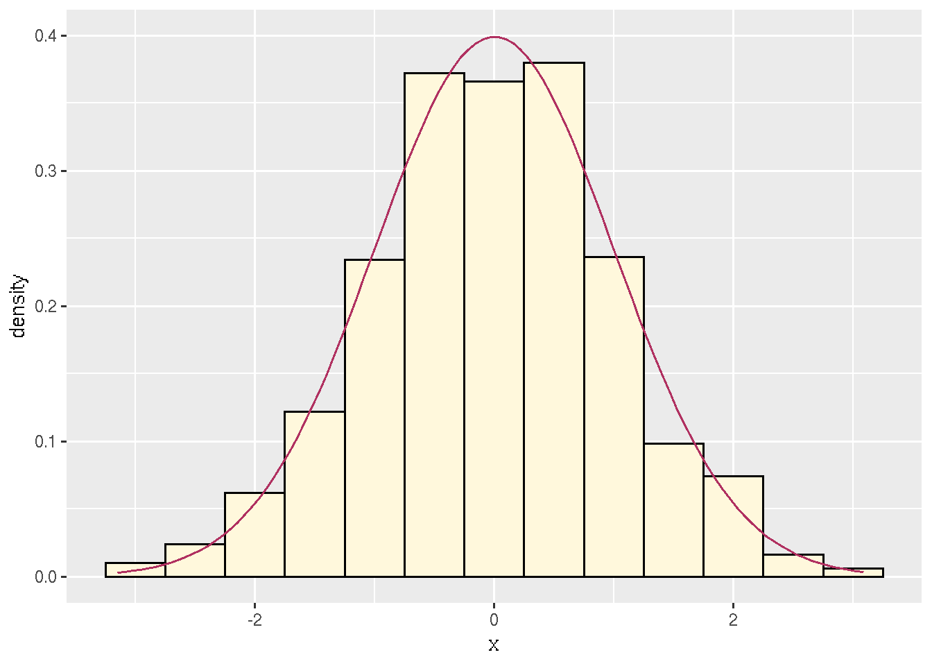
Figure 2.1: Histogram with probability density function.
The analog with base graphics doesn’t work as well because it is two commands that don’t talk to each other.
# for base graphics we don't need data in data frames
x <- mydata$x
hist(x, probability = TRUE)
curve(dnorm(x), add = TRUE)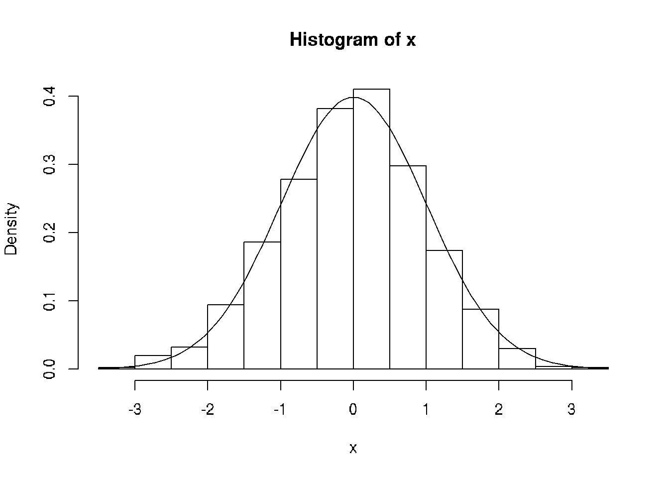
Figure 2.2: Histogram with probability density function (base graphics).
2.5.3 Tables
The no-snarf-and-barf rule means we have to use R to construct all our tables. To see how to do that, first we need a table.
Make up some regression data.
n <- 50
x <- seq(1, n)
a.true <- 3
b.true <- 1.5
y.true <- a.true + b.true * x
s.true <- 17.3
y <- y.true + s.true * rnorm(n)
And fit some models to it.
out1 <- lm(y ~ x)
out2 <- lm(y ~ x + I(x^2))
out3 <- lm(y ~ x + I(x^2) + I(x^3))
anova(out1, out2, out3)
## Analysis of Variance Table
##
## Model 1: y ~ x
## Model 2: y ~ x + I(x^2)
## Model 3: y ~ x + I(x^2) + I(x^3)
## Res.Df RSS Df Sum of Sq F Pr(>F)
## 1 48 16698
## 2 47 16659 1 39.03 0.1191 0.73161
## 3 46 15076 1 1582.30 4.8278 0.03308 *
## ---
## Signif. codes: 0 '***' 0.001 '**' 0.01 '*' 0.05 '.' 0.1 ' ' 1That is a table of sorts.
In order to make that a table nicely formatted for the document we are making, first we have to figure out what the output of R function anova is and capture it so we can use it.
foo <- anova(out1, out2, out3)
class(foo)
## [1] "anova" "data.frame"It is a data frame, which is the easiest thing to turn into a table, and the simplest way to do that seems to be the kable option on our R chunk
| Res.Df | RSS | Df | Sum of Sq | F | Pr(>F) |
|---|---|---|---|---|---|
| 48 | 16697.7 | ||||
| 47 | 16658.7 | 1 | 39.03 | 0.119 | 0.732 |
| 46 | 15076.4 | 1 | 1582.30 | 4.828 | 0.033 |
2.5.4 In-Line R
You can also execute R not in a code chunk but just in-line in your writing. Here is an example of that. First let’s get some computation we want to quote.
summary(out3)##
## Call:
## lm(formula = y ~ x + I(x^2) + I(x^3))
##
## Residuals:
## Min 1Q Median 3Q Max
## -34.83 -11.88 -0.29 11.00 47.72
##
## Coefficients:
## Estimate Std. Error t value Pr(>|t|)
## (Intercept) -15.639665 11.059835 -1.414 0.16407
## x 5.027970 1.859524 2.704 0.00957 **
## I(x^2) -0.177941 0.084274 -2.111 0.04020 *
## I(x^3) 0.002388 0.001087 2.197 0.03308 *
## ---
## Signif. codes: 0 '***' 0.001 '**' 0.01 '*' 0.05 '.' 0.1 ' ' 1
##
## Residual standard error: 18.1 on 46 degrees of freedom
## Multiple R-squared: 0.6261, Adjusted R-squared: 0.6017
## F-statistic: 25.67 on 3 and 46 DF, p-value: 6.576e-10The coefficients for x2 and x3 are not statistically significant, as shown by the ANOVA table. What they actually were was \(-0.177941\) and \(0.0023881\). Magic!
Note that these are coefficients for a regression on random data that is different every time the document is run (although wouldn’t be if we uncommented the set.seed command). By not using snarf-and-barf we always have the right numbers.
Also note that R Markdown (in its wisdom or unwisdom) forces you to know a little bit of LaTeX. When the number needs “scientific notation” R Markdown emits LaTeX here so the number must be enclosed in dollar signs (the LaTeX math marker for in-line math). So if these weren’t enclosed in dollar signs nonsense would be printed.
2.5.5 R Chunk Options
We have already illustrated a few R chunk options.
Another useful one is echo = FALSE. In this paragraph there is such a code chunk, but you don’t see it.
That is, you don’t see it unless you look at the source.
But we can use it in another code chunk.
hide## [1] 6.283185Any knitr chunk option found at https://yihui.name/knitr/options/ can be used as an R Markdown chunk option (knitr underlies rmarkdown).
Another useful option is cache = TRUE. That will be illustrated in the next chapter.